Quickstart
Installation
While installing DiffeRT2d and its dependencies on your global Python is fine, we recommend using a virtual environment (e.g., venv) for a local installation.
Dependencies
DiffeRT2d uses JAX for automatic differentation, which in turn may use (or not) CUDA for GPU acceleration.
If needed, please refer to JAX’s installation guidelines for more details.
Pip Install
The recommended way to install the latest release is to use pip:
pip install differt2d
Install From Repository
An alternative way to install DiffeRT2d is to clone the git repository, and install from there: read the contributing guide to know how.
Creating your first scene
DiffeRT2d is meant to perform Ray Tracing simulations on two dimensional scenes.
A scene is simply defined as a collection of objects
(see Object),
and some transmitters / receivers (see Point).
By default, DiffeRT2d only provides a few basic objects
(like straight walls, see Wall), but anyone
can create more complex objects, as long as the correct protocols are
implemented.
A few scenes are already provided with this library, and can be created with one-liner class methods, e.g.:
from differt2d.scene import Scene

scene = Scene.square_scene()
Modifying a scene
Objects can easily be added to a scene, and we use jax.numpy for
internal arrays storage. JAX provides the same API as numpy,
with additional utilities regarding automatic differention, which is
pretty useful for optimization problems.
import jax.numpy as jnp

from differt2d.geometry import Wall

wall = Wall(xys=jnp.array([[0.8, 0.2], [0.8, 0.8]]))
scene = scene.add_objects(wall)
Warning
Most classes are immutable PyTrees, meaning that mutation is performed by returning a new class instance.
Plotting utils
For testing purposes, most classes implement the
Plottable protocol, which means
you can easily plot a scene (and other objects) to see how it renders:
import jax.numpy as jnp
import matplotlib.pyplot as plt

from differt2d.geometry import Wall
from differt2d.scene import Scene

ax = plt.gca()
scene = Scene.square_scene()
wall = Wall(xys=jnp.array([[.8, .2], [.8, .8]]))
scene = scene.add_objects(wall)
scene.plot(ax)
plt.show()
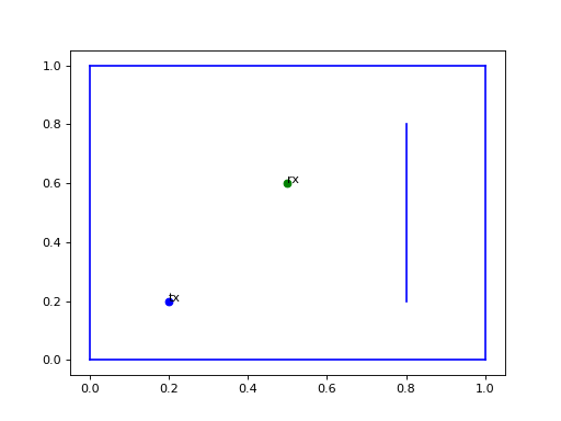
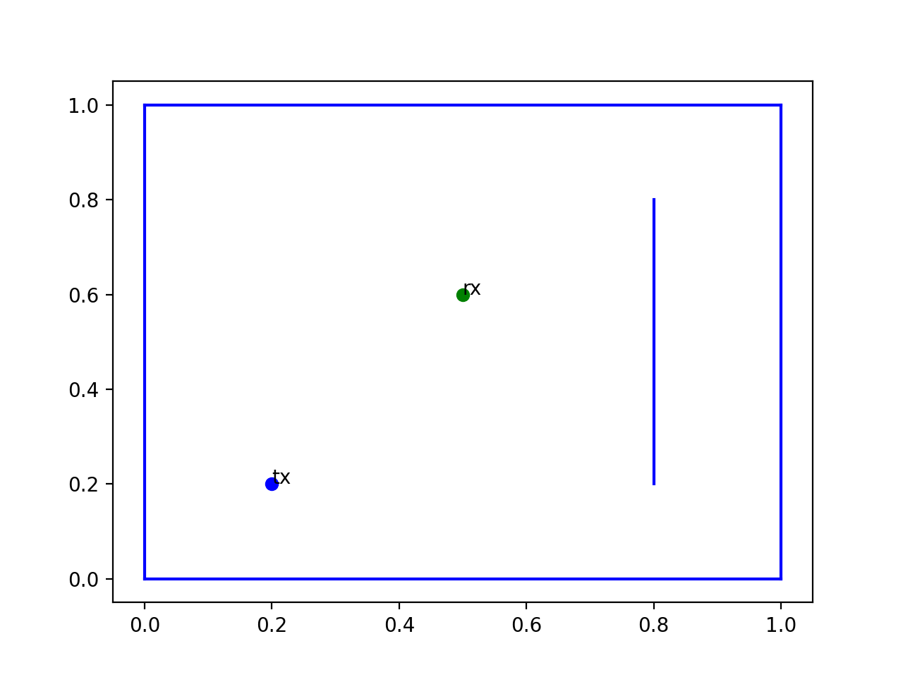
(Source code, png, hires.png, pdf)
If you need to, you can directly load any scene from OpenStreetMap using
Scene.from_geojson.
Tracing rays
Of course, this would not be a Ray Tracing module without some Ray Tracing tools!
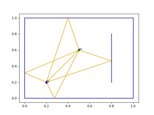
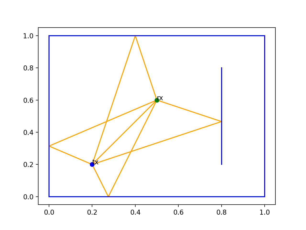
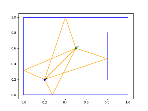
The easiest way to trace all paths from every transmitter to every receiver is to use
Scene.all_valid_paths:
import jax.numpy as jnp
import matplotlib.pyplot as plt

from differt2d.geometry import Wall
from differt2d.scene import Scene

ax = plt.gca()
scene = Scene.square_scene()
wall = Wall(xys=jnp.array([[.8, .2], [.8, .8]]))
scene = scene.add_objects(wall)
scene.plot(ax)

for _, _, path, _ in scene.all_valid_paths():
    path.plot(ax, zorder=-1)  # -1 to draw below the scene objects

plt.show()
(Source code, png, hires.png, pdf)
Power map
Maybe you are interested in determining the coverage of some antenna configuration?
For this purpose, you can easily accumulate some function, like the received power, on a grid and plot it:
import jax.numpy as jnp
import matplotlib.pyplot as plt

from differt2d.geometry import Wall
from differt2d.scene import Scene
from differt2d.utils import received_power

ax = plt.gca()
scene = Scene.square_scene()
wall = Wall(xys=jnp.array([[.8, .2], [.8, .8]]))
scene = scene.add_objects(wall)
scene.plot(ax, receivers=True)

X, Y = scene.grid(300)
Z = scene.accumulate_on_receivers_grid_over_paths(
    X,
    Y,
    fun=received_power,
    reduce_all=True
)
ax.pcolormesh(X, Y, 10.0 * jnp.log10(Z), zorder=-1)
plt.show()
(Source code, png, hires.png, pdf)
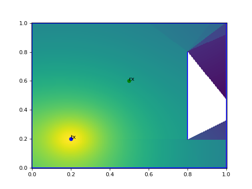
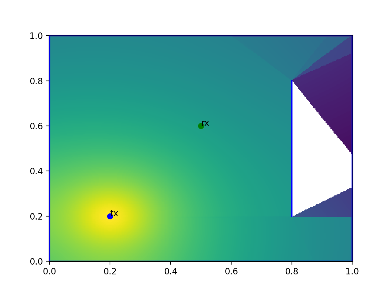
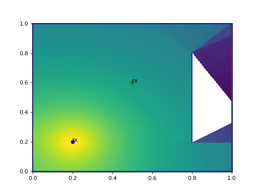
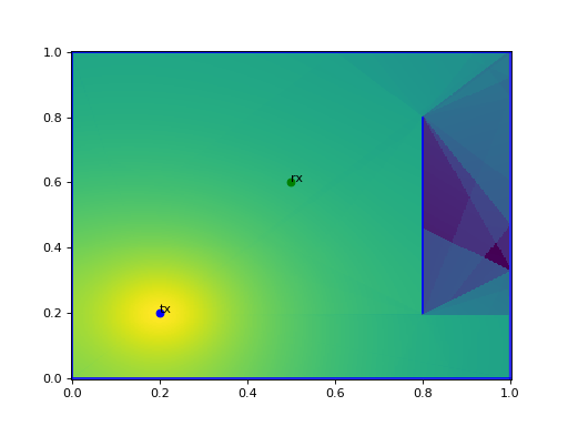
The above plot shows, for every possible receiver position in the scene, the received power transmitted by the transmitter. One can clearly see a shadowed region on the right of the scene, caused by the wall we just added. Of course, this region would receive some power if we were to simulate a higher order of interaction, e.g.:
import jax.numpy as jnp
import matplotlib.pyplot as plt

from differt2d.geometry import Wall
from differt2d.scene import Scene
from differt2d.utils import received_power

ax = plt.gca()
scene = Scene.square_scene()
wall = Wall(xys=jnp.array([[.8, .2], [.8, .8]]))
scene = scene.add_objects(wall)
scene.plot(ax, receivers=True)

X, Y = scene.grid(300)
Z = scene.accumulate_on_receivers_grid_over_paths(
    X,
    Y,
    fun=received_power,
    reduce_all=True,
    max_order=2  # The default value was 1
)
ax.pcolormesh(X, Y, 10.0 * jnp.log10(Z), zorder=-1)
plt.show()
(Source code, png, hires.png, pdf)
Power gradient
Because we use JAX almost everywhere in the code, taking gradient of functions
becomes straightforward, with jax.grad or jax.value_and_grad.
To make it easy, we also provide grad and value_and_grad options in
both
Scene.accumulate_on_transmitters_grid_over_paths
and
both
Scene.accumulate_on_receivers_grid_over_paths.
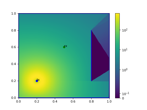
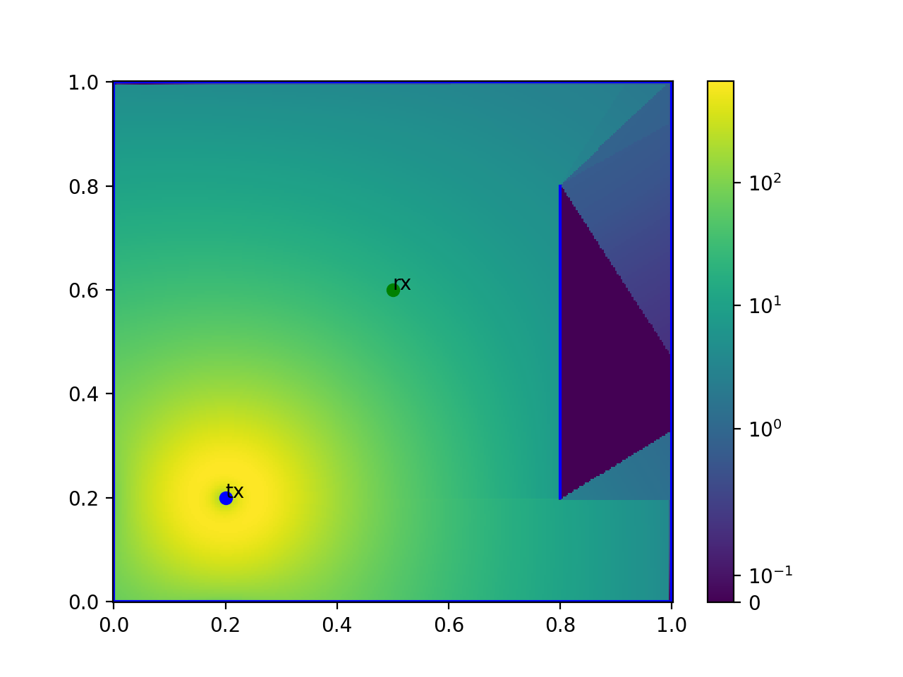
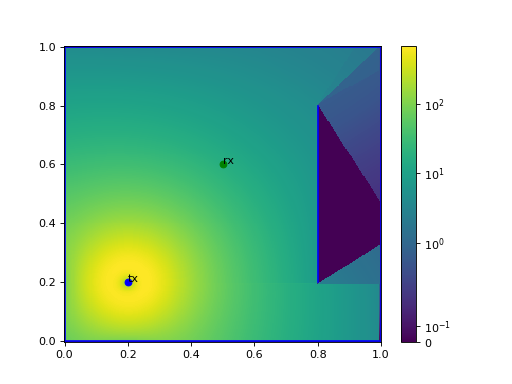
import jax.numpy as jnp
import matplotlib.pyplot as plt
from matplotlib.colors import SymLogNorm

from differt2d.geometry import Wall
from differt2d.scene import Scene
from differt2d.utils import received_power

fig, ax = plt.subplots()
scene = Scene.square_scene()
wall = Wall(xys=jnp.array([[0.8, 0.2], [0.8, 0.8]]))
scene = scene.add_objects(wall)
scene.plot(ax, receivers=True)

X, Y = scene.grid(300)
dZ = scene.accumulate_on_receivers_grid_over_paths(
    X,
    Y,
    fun=received_power,
    reduce_all=True,
    grad=True,
)
ndZ = jnp.linalg.norm(dZ, axis=-1)  # Norm of gradient
ndZ = jnp.nan_to_num(ndZ)  # NaN can arise from grad
im = ax.pcolormesh(
    X,
    Y,
    ndZ,
    norm=SymLogNorm(0.5, vmin=ndZ.min(), vmax=ndZ.max()),
    zorder=-1,
)
fig.colorbar(im, ax=ax) # Useful because non-linear scale
plt.show()
(Source code, png, hires.png, pdf)
More examples
For more usage examples, see the Examples Gallery section.